Finite methods
IMPORTANT Some of these functions require the Symbolic Math Toolbox to work. Make sure it is installed before trying to use them.
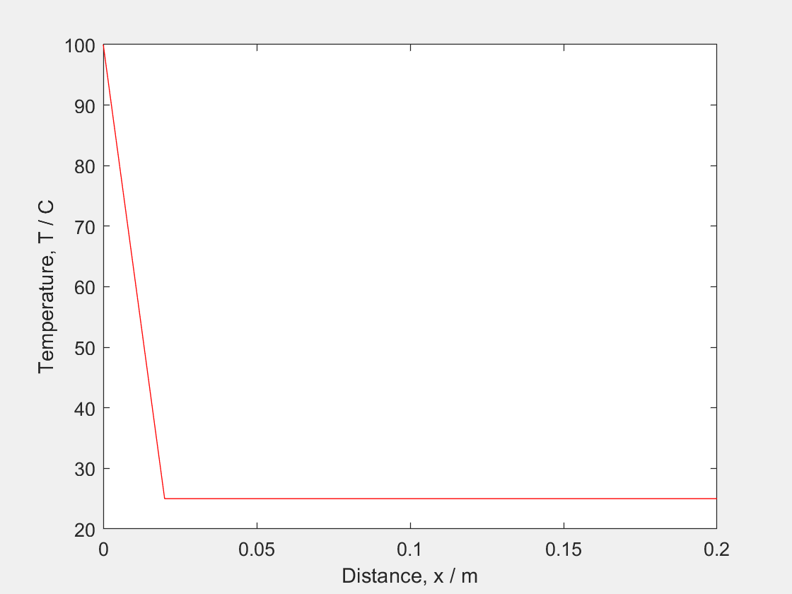
In the following example, it will be shown how to simulate a 1 Dimensional diffusion equation on an aluminum bar at room temperature with a constant heat source at 100 degrees on one of the ends.
\[\frac{\partial T}{\partial t} = \alpha \frac{\partial^2 T}{\partial x^2}\]Using the forward time difference approximation and the second spatial derivative approximation.
\[\frac{\partial T(t,x)}{\partial t} \approx \frac{T(t + \Delta t, x) - T(t,x)}{\Delta t}\] \[\frac{\partial^2 T(t,x)}{\partial x^2} \approx \frac{T(t,x +\Delta x) - 2T(t,x) + T(t,x - \Delta x)}{\Delta x^2}\]We can sub them back in and re-arrange it.
\[\frac{T(t + \Delta t, x) - T(t,x)}{\Delta t} \approx \alpha \frac{T(t,x +\Delta x) - 2T(t,x) + T(t,x - \Delta x)}{\Delta x^2}\] \[T(t+ \Delta t, x) \approx \alpha \frac{\Delta t}{\Delta x^2} [ T(t,x + \Delta x) - 2T(t,x) + T(t,x-\Delta x)] + T(t,x)\]And we can define sigma to merge all the constants and expand the expression.
\[T(t+\Delta t,x) \approx \sigma T(t,x+\Delta x) + \sigma T(t,x - \Delta x) + (1 - 2\sigma)T(t,x)\]- So we can starting expressing the constants: Alpha is the thermal diffusivity, a duration in hours, a length in metres, delta_x in metres and delta_t in seconds.
alpha = 5e-4; duration = 6; length = 0.1; delta_x = 0.01; delta_t = 0.1; t = 1; -
We then calculate the dimensions for the matrix and sigma. (If sigma is greater than 0.5 the simulation will become unstable)
steps_t = duration * 3600/delta_t+1; steps_x = length/delta_x+1; sigma = alpha*delta_t/delta_x^2 -
The next step is to set the initial conditions into the matrix
Temp = 25*ones(steps_t,steps_x); Temp(:,1) = 100; - We set up the plotting settings.
figure h = plot(0:delta_x:length,Temp(t,:),"-r"); xlabel('Distance, x / m') ylabel('Temperature, T / C') - Finally we create a loop to calculate the new values of the T throughout time.
 for t = 1:steps_t
     Temp(t+1,2:end-1) = sigma*Temp(t,1:end-2) + (1-2*sigma)*Temp(t,2:end-1)+ sigma*Temp(t,3:end);
     set(h,"YData",Temp((t+1),:))
     drawnow
 end