Return to Contents
Chapter 14 - Partial Differential Equations
This is an updated version of the notes, with a focus on the step-by-step process of analysing PDEs. To see the previous version, look in the PDF notes.
14.1 Recap
In chapter 8, we looked at ODEs – Ordinary Differential Equations. Here we had a quantity of interest, a model for how the system evolves in time, and a set of initial conditions. One of the examples that we considered was the trolley on a spring. Here the
- Quantity of interest : the position of the trolley at any moment in time $x(t)$
- Model for how it evolves : an ODE such as $\ddot{x}(t) = -\frac{k}{m} x(t)$,
- Initial conditions : $x(0)$ and $\dot{x}(0)$,the position and velocity of the trolley at $t=0$, when we start the clock.
Solving the ODE meant finding an $x(t)$ that satisfied the ODE in the general case (of any initial conditions), i.e. $x(t) = A \cos(\omega t) + B \sin(\omega t)$ with $\omega = \sqrt{\frac{k}{m}}$; then matching this general solution to the particular initial conditions we were given. i.e. $x(t) = x(0) \cos(\omega t) + \frac{\dot{x}(0)}{\omega}\sin{\omega t}$.
Next, we considered Coupled Oscillators, which took a similar approach, but we had multiple discrete quantities of interest, and again a model for how the system evolves and set of initial conditions. E.g. for a set of trolleys connected to each other with springs.
In this setup we upgraded some of our quantities to vectors and matrices, e.g. $x(t) \rightarrow \mathbf{x}(t)$, and our ODE became,
\[\ddot{\mathbf{x}}(t) = \begin{bmatrix} -\frac{k_1 + j}{m_1} & \frac{j}{m_1} \\ \frac{j}{m_2} & -\frac{k_2 + j}{m_2} \end{bmatrix} \mathbf{x}\]We solved this system by finding the normal modes that oscillate in harmonic motion at a single frequency, and added the combination of all solutions together for the genaral solution, before matching to initial conditions.
14.1.1 Upgrading to PDEs
Partial Differential Equations, PDEs, are the next step in this progression where we go from modelling the time evolution of single quantity (ODE), to a discrete set of quantities (CHO), to a continuous set of values. Some examples of these situations include the displacement of every point on a guitar string when it is struck, the temperature at every point in a room when a heat source is nearby, the stresses on any part of the body of an aircraft during operation.
Solving PDEs allows us to calculate how our systems evolve in time, but also can give us insight into how to optimise them e.g. for their response efficiency, or to detect failure modes.
PDEs find applications in many fields of Engineering, and are studied in their own right as a topic in Applied Mathematics. In this module we will introduce the topic and give a first set of tools for approaching them.
We will be relying heavily on the intuition you have built up for ODEs, so make sure you are refreshed and comfortable with that topic.
14.2 Introducing PDEs
Returning to our analogy of ODEs and Coupled Oscillators, our quantity of interest is usually the value of a quantity both at some moment in time and now also at some point in space. i.e. a multivariate function of space and time – $f(\mathbf{x}, t)$.
The model for our system, how our quantity of interest evolves in time, is no longer an Ordinary Differential Equation, but a Partial Differential Equation, i.e. a differential equation that contains partial derivatives.
Some physically motivated PDEs that we’ll look at in more detail are:
The diffusion equation:
\[\frac{\partial f(x, t)}{\partial t} = \alpha \frac{\partial^2 f(x, t)}{\partial x^2}\]And the wave equation:
\[\frac{\partial^2 f(x, t)}{\partial t^2} = c^2 \frac{\partial^2 f(x, t)}{\partial x^2}\]Notice that in each we have derivatives in both space and time of our quantity of interest, $f(x, t)$, as well as some constants of the system, $\alpha$ and $c$.
One thing to be aware of, is previously our quantity of interest was labeled $x$, and we solved for $x(t)$. Now, our quantity of interest is $f(…)$ and now $x$ is one of our independent variables along with $t$, and we solve for $f(x, t)$. In different applications, we may use different symbols for our dependent and independent quantities, so it’s always worth noting which variables play what role.
The initial conditions of the system also upgrade, instead of just a single value when $t=0$, we now typically specify an entire function, $f(x, 0)$ – i.e. what the system looks like at a snapshot in time.
Solving partial differential equations amounts to asking the question:
“If I have a system who’s behaviour is governed by a particular PDE, and the system starts with a known initial state: What is the state of the system at future times?”
14.2.1 1D Wave Equation Example
In general, PDEs are difficult to solve. We will focus primarily on two special cases that have special relevance in engineering and are tractable to solve. The tools and methods of analysis will allow you to analyse a wider class of problems.
The wave equation is a class of PDEs that models vibration and wave phenomena. This can be applied to multiple physical systems from mechanical vibrations in solid bodies, to sound waves in acoustic systems, and electromagnetic waves – i.e. light.
We saw a wave equation earlier in this chapter that looked like this,
\[\frac{\partial^2 f(x, t)}{\partial t^2} = c^2 \frac{\partial^2 f(x, t)}{\partial x^2}\]One question we may wish to answer when we have a PDE is, “Do I have a particular function that solves this PDE?”. If we have a candidate function $f(x, t) = \operatorname{sech}(x - a t)$, where $a$ is a constant term, let’s determine if this solves the PDE (we can discuss how we would get such a function later)
First thing to do is to calculate the derivatives of $f(x, t)$ that appear in the PDE. In this case, the second derivatives in space and time. (This can be done by hand, but Wolfram Alpha is pretty good for this too.)
\[\begin{align*} \frac{\partial f(x, t)}{\partial x} &= -\tanh(x - a t)\operatorname{sech}(x - a t) \\ \frac{\partial^2 f(x, t)}{\partial x^2} &= \operatorname{sech}(x - a t) - 2\operatorname{sech}^3(x - a t) \\ \frac{\partial f(x, t)}{\partial t} &= a \tanh(x - a t)\operatorname{sech}(x - a t) \\ \frac{\partial^2 f(x, t)}{\partial t^2} &= a^2 \operatorname{sech}(x - a t) - 2 a^2 \operatorname{sech}^3(x - a t) \end{align*}\]Then if we insert these derivatives into the PDE, the original wave equation, we can cancel things down,
\[a^2 \operatorname{sech}(x - a t) - 2 a^2 \operatorname{sech}^3(x - a t) = c^2 \left(\operatorname{sech}(x - a t) - 2\operatorname{sech}^3(x - a t)\right)\]which reduces to,
\[a^2 = c^2\]This shows we have a condition on $f(x, t) = \operatorname{sech}(x - a t)$ being a solution. It is a solution, if and only if $a^2 = c^2$, i.e., $a = \pm c$. Physically, this tells us the speed of the function, that the $\operatorname{sech}$ envelope travels at speed $c$, which was one of the constants of the PDE.
Therefore we have two solutions to the wave equation, $f(x, t) = \operatorname{sech}(x - c t)$ and $f(x, t) = \operatorname{sech}(x + c t)$. The wave equation is a linear differential equation, which means we can combine any two solutions to form a third new solution – recall how this was the case with ODEs as well. So a more general solution to the PDE is,
\[f(x, t) = A\operatorname{sech}(x - c t) + B\operatorname{sech}(x + c t)\]This is good, and we’ve made progress, however we’re not yet confident we’ve found all solutions – what if our function doesn’t look like $\operatorname{sech}$? The following functions also solve the wave equation,
\[\begin{align*} f(x, t) &= e^{-(x - c t)^2 / w^2} \\ f(x, t) &= \frac{1}{w^2 + x^2 + 2 x c t + c^2 t^2} \end{align*}\]where $w$ is a free parameter that controls the width. Try yourself by inserting these into the differential equation.
Since these solve the PDE with any value of parameter, $w$, then any sum of solutions is also a solution, e.g.,
\[f(x, t) = \sum_w A_w e^{-(x - c t)^2 / w^2} + B_w \frac{1}{w^2 + x^2 + 2 x c t + c^2 t^2}\]for a set of $w$ values.
The solutions above were given - we just verified they worked. It would be good to have a more systematised way to approach the PDEs.
(It turns out with the 1D wave equation that any function, $f(x, t) = f_+(x - c t) + f_-(x + c t)$, is a solution, for arbitrary $f_+(x)$ and $f_-(x)$. This is a special case though, we need something that will work in general.)
14.3 Separation of Variables
Let’s trial another solution to the wave equation,
\[f(x, t) = \cos k x \cos \omega t\]Here the parameter $k$ is called the wavevector and it determines the wavelength of the cosine, $l = 2\pi / k$. The parameter $\omega$ is the angular frequency (or informally just frequency) and determines the time period, $\tau = 2\pi / \omega$. If we insert this into the wave equation, we get the result,
\[\begin{align*} \frac{\partial^2 }{\partial t^2} \cos k x \cos \omega t &= c^2 \frac{\partial^2}{\partial x^2} \cos k x \cos \omega t \\ {-} \omega^2 \cos k x \cos \omega t &= {-} c^2 k^2 \cos k x \cos \omega t \end{align*}\]And therefore,
\[\omega^2 = c^2 k^2\]This resulting equation is called the dispersion relation, which sets the relationship between the frequency and the wavevector that is the condition for $f(x, t)$ to be a solution to the wave equation. It says that a sinusoidal wave with a specific wavelength has a fixed period that is related to it.
Let’s look into our solution and see if there are any general lessons we can learn. Our trial solution, $f(x, t) = \cos k x \cos \omega t$, had relatively simple derivatives. Part of the reason for this is the part of the expression that varies in $x$, i.e. $\cos k x$, and the part that varies in $t$, i.e. $\cos \omega t$, are multiplied together, rather than mixed in a more intricate manner.
14.3.1 Procedure
This is a key insight, we can look for solutions where the variables, $x$ and $t$, are separated in multiplied terms. This technique is called Separation of Variables Let’s imagine we have a solution to the wave equation, $f(x)$, which is the product of a part that only varies in $x$, let’s call that part $X(x)$, and a part that only varies in $t$, lets call that $T(t)$, then we express our solution as $f(x) = X(x)T(t)$.
What happens if we plug this into the wave equation.
\[\begin{align*} \frac{\partial^2 f(x, t)}{\partial t^2} &= c^2 \frac{\partial^2 f(x, t)}{\partial x^2} \\ \frac{\partial^2}{\partial t^2} X(x)T(t) &= c^2 \frac{\partial^2}{\partial x^2} X(x)T(t) \end{align*}\]Now the partial derivatives only see, therefore affect their respective terms, i.e.,
\[X(x) \left(\frac{\partial^2}{\partial t^2} T(t)\right) = c^2 \left(\frac{\partial^2}{\partial x^2} X(x) \right)T(t)\]which we can shorthand to,
\[X(x)T^{\prime\prime}(t) = c^2 X^{\prime\prime}(x)T(t)\]To make this more manageable, we divide both sides by $X(x)T(t)$,
\[\frac{X(x)T^{\prime\prime}(t)}{X(x)T(t)} = c^2 \frac{X^{\prime\prime}(x)T(t)}{X(x)T(t)}\]Cancelling terms returns,
\[\frac{T^{\prime\prime}(t)}{T(t)} = c^2 \frac{X^{\prime\prime}(x)}{X(x)}\]By taking one of the terms, $T^{\prime\prime}(t) / T(t)$, you can see it is only dependant on $t$. The other term, $X^{\prime\prime}(x) / X(x)$, is only dependant on $x$. The big step conceptually from here is to recognise that since the $t$ term must be equal to a set of other terms that don’t involve $t$, the $t$ term itself must be independent of $t$, i.e. is a constant:
\[\frac{T^{\prime\prime}(t)}{T(t)} = a \,,\]where $a$ is a constant. And this can be re-arranged into,
\[T^{\prime\prime}(t) = a T(t)\]i.e. a linear ODE.
The same is true of the $x$ term.
\[X^{\prime\prime}(x) = b X(x)\]where $b$ is also a constant, with the relationship $a = c^2 b$ linking the two.
14.3.2 Reflection
Let’s pause here. What we have done is to convert a PDE, which in principle is difficult to solve,
\[\frac{\partial^2 f(x, t)}{\partial t^2} = c^2 \frac{\partial^2 f(x, t)}{\partial x^2}\]into two ODEs, a relationship between their constants, and a recipe for the PDE solution built out of the ODE solutions.
\[\begin{align*} T^{\prime\prime}(t) &= a T(t) \\ X^{\prime\prime}(x) &= b X(x) \\ a &= c^2 b \\ f(x) &= X(x)T(t) \end{align*}\]From here we can tackle the ODEs using the tools developed in a previous chapter.
14.3.3 Tackling the ODEs
Our ODEs here in $x$ and $t$ take the same form, First, focus on the $x$ one.
\[X^{\prime\prime}(x) = b X(x)\]Reading the ODE, it is asking, ‘what function, when differentiated twice, returns itself times a constant?’ Exponential functions fit the bill here, and so do sines and cosines if $b$ is negative. We’re free to choose, let’s look at sines and cosines as we saw them before.
Let’s use the trial function,
\[X(x) = \sin k x\]If we insert it into the ODE, we get,
\[{-}k^2 \sin k x = b \sin k x\]or
\[{-}k^2 = b\]i.e.¸
\[X(x) = \sin \left(\sqrt{-b} x \right)\]The same is true of $X(x) = \cos \left(\sqrt{-b} x \right)$. So we can write a combined solution,
\[X(x) = A \sin \left(\sqrt{-b} x \right) + B \cos \left(\sqrt{-b} x \right)\]We could do the same with $t$ for,
\[T(t) = C \sin \left(\sqrt{-a} t \right) + D \cos\left(\sqrt{-a} t \right)\]Giving a combined solution that is the product of the separated solutions:
\[f(x, t) = \left[A \sin \left(\sqrt{-b} x \right) + B\cos \left(\sqrt{-b} x \right)\right] \left[C \sin \left(\sqrt{-a} t \right) + D\cos \left(\sqrt{-a} t \right)\right]\]Which you can check solves the full PDE.
Give this a go yourself in the tutorial sheet.
14.3.4 Better constants
The square roots aren’t very nice here, but since $a$ and $b$ are arbitrary constants (they could be positive, negative, complex), we can replace them with more meaningful symbols. This assists in an easier ability to simply look at the function and understand what it is doing, as well as being nicer to look at. We used $k^2 = -b$ earlier as the coefficient of $x$. If we replace all instances of $b$ with $-k^2$, and similarly $a$ with $-\omega^2$, We get as our solution,
\[f(x, t) = \left[A \sin \left(k x \right) + B\cos \left(k x \right)\right] \left[C \sin \left(\omega t \right) + D\cos \left(\omega t \right)\right]\]Or if we use the aforementioned dispersion relation, we get:
\[f(x, t) = \left[A \sin \left(k x \right) + B\cos \left(k x \right)\right] \left[C \sin \left(k c t \right) + D\cos \left(k c t \right)\right]\]This shows shorter wavelengths we have a higher frequency.
More crucially, if we replace our ODEs with,
\[\begin{align*} T^{\prime\prime}(t) &= -\omega^2 T(t) \\ X^{\prime\prime}(x) &= -k^2 X(x) \\ \omega^2 &= c^2 k^2 \\ f(x) &= X(x)T(t) \end{align*}\]If we had anticipated the result, we could have called our arbitrary complex constants $-k^2$ and $-\omega^2$ this way from the start. Here $k$ and $\omega$ are the wavevector and (angular) frequency that we met earlier.
Note how we have freedom to choose the names of our arbitrary constants. If we had set $T^{\prime\prime}(t) = \gamma^2 T(t)$ and $X^{\prime\prime}(x) = \kappa^2 X(x)$ this would show exponentially growing and decaying solutions. How would this affect the dispersion relation? Try this question.
As a rule, to choose constants, you want to set the power to be the same as the highest order derivative in your ODE. Then to choose if you want a positive or a negative sign, if you’ve got a 1st order ODE, a negative sign will return an exponentially decaying function, and a positive sign returns an exponentially growing function. if you’ve got a 2nd order ODE, a negative sign will return oscillatory solutions, whereas a positive sign will return decaying and growing solutions. Usually you want your time function to decay into the future, and then your spatial parts can be set to keep the values of your constants positive in the dispersion relation.
14.3.5 Summary of Separation of Variables
Let’s pause again and reflect. We’ve managed to derive the sinusoidal solution that we guessed earlier, but this time from first principles.
What was our process?
- Assume a solution that is separable, e.g., $f(x, t) = X(x)T(t)$.
- Plug this into our PDE, and let the derivatives work on like terms.
- Divide the whole thing by $X(x)T(t)$ and collect like terms.
- Set these terms to be constant, to define ODEs and a dispersion relation.
- Solve the ODEs and combine the solutions together.
We’ll see in the next section this working on a different set of PDEs.
14.4 Diffusion Equation
The diffusion equation is for diffusion processes, i.e. how a concentration of a substance spreads out through a medium. This could be how Lithium ions in an energy fuel cell diffuse through a porous medium. It is also the equation that governs temperature, and how heat is transfered through solids. For this reason, the diffusion equation is also called the Heat Equation.
The 1D diffusion has the form,
\[\frac{\partial u}{\partial t} = \alpha \frac{\partial^2 u}{\partial x^2}\]Where $u$ is the diffusing quantity, and $\alpha$ is the diffusivity, a measure of how quickly the substance diffuses.
If we try to interpret the PDE, it’s saying the concentration of a substance will change over time in proportion to the local curvature (2nd derivative). Or if there’s more concentration on average adjacent to a point, then over time the concentration will flow to average out and come to equilibrium.
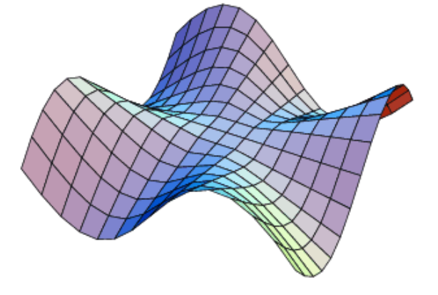
Here is a plot of one of the solutions to the diffusion equation, to give you a feel for the dynamics.
Let’s use Separation of Variables to solve the diffusion equation.
- Assume a solution that is separable.
- Plug this into our PDE, and let the derivatives work on like terms.
- Divide the whole thing by $X(x)T(t)$ and simplify.
-
Set these terms to be constant, to define ODEs and a dispersion relation.
For $x$, we’ve seen this before and can set $X^{\prime\prime}(x) / X(x) = -k^2$, choosing $-k^2$ to be our constant, which will imply sinusoidal solutions. This returns the ODE $X^{\prime\prime}(x) = -k^2 X(x)$.
For $t$, let’s use $T^{\prime}(t) / T(t) = -\gamma$, the minus sign isn’t strictly needed, but we’ll see turns out to be the best choice. The second ODE is therefore, $T^{\prime}(t) = -\gamma T(t)$ and the dispersion relation is $\gamma = \alpha k^2$. (showing if $k$ is real then $\gamma$ is positive). -
Solve the ODEs and combine the solutions together.
The $X(x)$ part has the solutions we saw before,
$X(x) = A \sin \left(k x \right) + B\cos \left(k x \right)$
The $T(t)$ part is a first order ODE, so only has one solution,
$T(t) = e^{-\gamma t}$
giving a full solution,
When we insert the dispersion relation, we get,
\[U(x, t) = A \sin \left(k x \right) e^{-\alpha k^2 t} + B\cos \left(k x \right) e^{-\alpha k^2 t}\]Which should match to our intuition, the sinusoids that have the shortest periods decay away the quickest.
14.5 Further Examples
We’ve so far looked at the 1D Undamped Wave Equation and 1D Diffusion Equation. It’s worth briefly looking into some extensions of these cases to see how the Separation of Variables methods generalises.
14.5.1 2D Diffusion Equation
Let us now introduce higher dimension PDEs.Often PDEs generalise by replacing their spatial $\frac{\partial^2}{\partial x^2}$ term with the Laplacian, $\nabla^2$. The 2D Diffusion equation for example looks like,
\[\frac{\partial u(x, y, t)}{\partial t} = \alpha \nabla^2 u(x, y, t)\]We solve this in a very similar to the 1D case. Let’s assume our trial solution is,
\[u(x, y, t) = X(x)Y(y)T(t)\]Then inputting into the 2D diffusion equation, we get,
\[\frac{T^{\prime}(t)}{T(t)} = \alpha \frac{X^{\prime\prime}(x)}{X(x)} + \alpha \frac{Y^{\prime\prime}(y)}{Y(y)}\]Each of the separated terms gets its own constant and ODE, and we get a dispersion relation linking them,
\[\begin{align*} T^{\prime}(t) &= -\gamma T(t) \\ X^{\prime\prime}(x) &= -k_x^2 X(x) \\ Y^{\prime\prime}(y) &= -k_y^2 Y(y) \\ \gamma &= \alpha \left( k_x^2 + k_y^2 \right) \end{align*}\]The ODEs can be solved and combined here as before.
Things to note are, we have two degrees of freedom in $k_x$ and $k_y$ which in turn determine the value of $\gamma$.
In the tutorial questions we find the solution in terms of complex exponentials.
14.5.2 Damped Wave Equation
Another equation we can look at is the damped wave equation, here in 1D. Thw below equation is the wave equation we’ve seen already but with a damping term that seeks to extinguish vibrations over time.
\[\frac{\partial^2 f(x, t)}{\partial t^2} = {-} 2g \frac{\partial f(x, t)}{\partial t} {+} c^2 \frac{\partial^2 f(x, t)}{\partial x^2}\]Where here $g$ is a newly introduced damping constant, that is the coefficient for a first derivative in $t$. We approach this as usual, i.e. $f(x, t) = X(x)T(t)$, and get,
\[\frac{T^{\prime\prime}(t)}{T(t)} = -2 g \frac{T^{\prime}(t)}{T(t)} + c^2 \frac{X^{\prime\prime}(x)}{X(x)}\]Now before we start assigning constants, we need to group together like terms. Our assumption previously was that our $t$ block is equal to things that don’t depend on $t$, this is only true if both $t$ terms are grouped together. i.e.,
\[\frac{T^{\prime\prime}(t) + 2 g T^{\prime}(t)}{T(t)} = c^2 \frac{X^{\prime\prime}(x)}{X(x)}\]Allowing us to write,
\[\begin{align*} T^{\prime\prime}(t) + 2 g T^{\prime}(t) &= -\omega^2 T(t) \\ X^{\prime\prime}(x) &= -k^2 X(x) \end{align*}\]Here, we still have $\omega^2 = c^2 k^2$. The $g$ term is wrapped up in the $T(t)$ ODE. This ODE is solved as seen previously.
14.6 Initial Conditions
So far we have found general solutions to PDEs, either by having a test solution and checking any constraints on it, or by using separation of variables to generate new solutions. In either case we were able to generate new solutions as a linear combination of other solutions.
What we would really like to be able to say is, “If our systems starts in this initial condition, how does it evolve into future times”. If our concentration starts over here, what does it do next?
Previously with ODEs, our initial condition was a set of values : i,e at $t=0$, the position, $x(t=0)$, and sometimes the velocity, $x’(t=0)$. For a second order ODE we needed two values, and for a first order one value, and this pattern repeats. For PDEs, our initial conditions are usually specified as the value of the function for every point in space at a single time, e.g. $f(x, y, t=0)$. If we can match our initial conditions to a solution when $t=0$ then we can know how the system will behave at future times.
14.6.1 1D Diffusion Equation
For example, let’s consider the 1D diffusion equation, We saw above that it has solutions,
\[U(x, t) = A \sin \left(k x \right) e^{-\alpha k^2 t} + B\cos \left(k x \right) e^{-\alpha k^2 t}\]Let’s assume here that we have a value for our diffusivity, $\alpha = 1 \, \mathrm{m}^2 / \mathrm{s}$ If we are told that at $t=0$, concentration of our substance is distributed as,
\[U_0(x) = 10\,\mathrm{g}/\mathrm{m}\; \cos \left(\frac{2 \pi}{0.5 \mathrm{m}} x \right)\]Then, we can pattern match our full solution to this, We can write our solution $t=0$ as,
\[U(x, t=0) = A \sin \left(k x \right) + B\cos \left(k x \right)\]Pattern matching, we can determine for $U(x, t=0) = U_0(x)$,
$A = 0$, $B = 10\,\mathrm{g}/\mathrm{m}$, and $k=2 \pi / 0.5 \, \mathrm{m}^{-1}$.
From here, carry outpattern matching, by comparing coefficients and looking for patterns. We can insert the parameters we have now determined into the full solution, giving,
\[U(x, t) = 10\,\mathrm{g}/\mathrm{m} \cos \left(\frac{2 \pi}{0.5 \mathrm{m}} x \right) \exp\left({-\frac{(2 \pi)^2}{0.25} \mathrm{s}^{-1} t}\right)\]or
\[U(x, t) = 10\,\mathrm{g}/\mathrm{m} \; \cos \left(12.6 \, \mathrm{m}^{-1} \; x \right) \exp\left({- 128 \, \mathrm{s}^{-1} \; t}\right)\]Which tells us what our system looks like at all times.
14.6.2 More Complex
In general, things are a little more complicated than this. The wave equation, for example, is second order in time. This means we need to specify not just initial values, but also inital time derivatives too. E.g., We can look at the 1D wave equation, that has solution,
\[f(x, t) = \left[A \sin \left(k x \right) + B\cos \left(k x \right)\right] \left[C \sin \left(k c t \right) + D\cos \left(k c t \right)\right]\]We might be told, at $t=0$ the value of the function is zero everywhere, $f_0(x) = 0$, but the time derivative has value $f^{(t)}_0(x) = 0.4 \sin 3 x$.
Here we need match our solution and its time derivative to our intial conditions at $t=0$. i.e.
\[\frac{\partial f}{\partial t}(x, t) = \left[A \sin \left(k x \right) + B\cos \left(k x \right)\right] \left[C k c \cos \left(k c t \right) - D k c\sin \left(k c t \right)\right]\]So at $t=0$,
\[\begin{align*} f(x, 0) &= \left[A \sin \left(k x \right) + B\cos \left(k x \right)\right] D \\ \frac{\partial f}{\partial t}(x, 0) &= \left[A \sin \left(k x \right) + B\cos \left(k x \right)\right] C k c \end{align*}\]If we pattern match, $f(x, 0) = 0$,
$D=0$,
then matching $\frac{\partial f}{\partial t}(x, 0) = f^{(t)}_0(x)$,
$B = 0$, $k=3$, $A C = 0.4 / (k c) = 0.133 / c$.
This gives full solution,
\[f(x, t) = 0.133 \sin \left(3 x \right)\sin \left(3 c t \right)\]14.6.3 Pattern Matching Multiple Solutions
Sometimes, the function we are matching to may not look exactly like our solution, e.g. for the diffusion equation, we may have an initial condition of,
\[u_0(x) = 4 \cos (2 x) + 7 \cos (3 x)\]Here we can pattern match each part of the sum separately, e.g. if our initial condition was,
\[u_0(x) = 4 \cos (2 x)\]then our full solution would be,
\[u(x, t) = 4 \cos (2 x) e^{-4 \alpha t}\]and equivalently, for an initial condition,
\[u_0(x) = 7 \cos (3 x)\]Our full solution is,
\[u(x, t) = 7 \cos (3 x) e^{-9 \alpha t}\]Since linearity applies, we can add these solutions together.
\[u(x, t) = 4 \cos (2 x) e^{-4 \alpha t} + 7 \cos (3 x) e^{-9 \alpha t}\]Which we can double check does indeed equal $4 \cos (2 x) + 7 \cos (3 x)$ when $t = 0$.
This is important to reflect on, sometimes we need to pattern match to a sum of solutions to the equation. In the cases we’ve seen the spatial wavevector, $k$, is a free parameter. It can take any value (even complex). So we’re free to add any form of this solution with a specific $k$ together to form a particular solution, as we saw in the previous example with $k = 2$ and $k = 3$.
We can write this more explicitly as follows, For the diffusion equation, we had solution,
\[U(x, t) = A \sin \left(k x \right) e^{-\alpha k^2 t} + B\cos \left(k x \right) e^{-\alpha k^2 t}\]Now, since $k$ is arbitrary, we can sum over different values of $k$. Each of these will have a different $A$ and $B$ coefficient, so we can label these with a subscript.
\[U(x, t) = \sum_k A_k \sin \left(k x \right) e^{-\alpha k^2 t} + B_k \cos \left(k x \right) e^{-\alpha k^2 t}\]This might look familiar from Fourier Series, and indeed in general, if you can match a function’s Fourier coefficients to the PDE solution at $t=0$, then this will tell you the evolution of that function under the PDE at future times.
14.7 Boundary Conditions
So far, we have been looking at solutions to the our PDEs that fill all space. I.e. there has been no constraint on what $x$ values are allowed. But, for example, if we have a wave on a guitar string, the string has a length and our solution is only valid on the length of the string.
14.7.1 Fixed value boundary conditions (Dirichlet)
Let’s say our guitar string has a length $L$, and waves on it are defined on $x \in [0, L]$. We can specify a boundary condition, which is how the system behaves on a boundary, in this case, at $x = 0$ and $x = L$. One such condition could be that the string is fixed in place at the boundary, i.e. $f(x=0, t) = 0$ and $f(x=L, t) = 0$, at all times.
Let’s incorporate these into the wave equation solution,
\[f(x, t) = \sum_k \left[A_k \sin \left(k x \right) + B_k\cos \left(k x \right)\right] \left[C_k \sin \left(k c t \right) + D_k\cos \left(k c t \right)\right]\]First, let’s set $x = 0$,
\[f(0, t) = B_k \left[C_k \sin \left(k c t \right) + D_k \cos \left(k c t \right)\right] = 0\]This implies that $B_k = 0$ for the function to be zero at all times. Next, let’s set $x = L$, here we get,
\[f(L, t) = \sum_k A_k \sin \left(k L \right) \left[C_k \sin \left(k c t \right) + D_k\cos \left(k c t \right)\right] = 0\]At this stage, we can’t set this to equal zero by setting any coefficients, (setting $A_k = 0$ would mean the function is zero everywhere at all times – a solution, but uninteresting). If the $\sin \left(k L \right)$ term was zero though, then the whole expression would be. What is the condition for a sine function to be zero? If its argument is an integer multiple of $\pi$, setting $k L = n \pi$, with $n \in \mathbb{Z}$, this works. This gives a condition on $k$, i.e. that $k = n \pi / L$. So instead of $k$ being any complex number, by imposing these boundary conditions, we’ve said that $k$ can only be discrete real values, i.e. our general solution after applying the boundary conditions becomes,
\[f(x, t) = \sum_{n=0}^{\infty} A_k \sin \left(\frac{n \pi x}{L} \right) \left[ C_k \sin \left(\frac{n \pi c t}{L} \right) + D_k\cos \left(\frac{n \pi c t}{L} \right) \right]\]We can actually tidy this up further, by redefining our coefficients,
\[f(x, t) = \sum_{n=0}^{\infty} \sin \left(\frac{n \pi x}{L} \right) \left[ a_n \sin \left(\frac{n \pi c t}{L} \right) + b_n\cos \left(\frac{n \pi c t}{L} \right) \right]\]Let’s review what we’ve just done. We’ve restricted our spatial range from an infinite range to a finite section, and this has had the result of quantising the allowed wavevectors of modes in the system. You’ll also notice that the frequency has been quantised too now, even though we’ve not restricted anything in time. This is because our dispersion relation holds, $\omega^2 = c^2 k^2$, hence $\omega = n \pi c / L$.
This is interesting in itself, because we can ask what the lowest frequency of the system is. We can get this by setting $n = 1$ (If we set $n=0$ we get zero everywhere). The fundamental frequency, lowest frequency, of the system is $\omega_1 = \pi c / L$, and all other frequencies are, in this case, integer multiples – or overtones – of the fundamental frequency, $\omega_n = n \omega_1$. This is what makes musical instruments sound the way they do. The geometry of the instrument constrains the smallest frequency it can produce to its lowest note, the note is then supplemented by overtones which give each instrument its own sound.
Boundary conditions where we set the value of the function like this are called Dirichlet boundary conditions.
14.7.2 Fixed derivative boundary conditions (Neumann)
In principle, we can also set boundary conditions where the derivative of the field is zero at the boundary. These are called Neumann boundary conditions. Let’s have a look at this one, Formally $f^{(x)}(x=0, t) = 0$ and $f^{(x)}(x=L, t) = 0$. Using the general solution again,
\[f(x, t) = \sum_k \left[A_k \sin \left(k x \right) + B_k\cos \left(k x \right)\right] \left[C_k \sin \left(k c t \right) + D_k\cos \left(k c t \right)\right]\]The spatial derivative of this is,
\[f^{(x)}(x, t) = \sum_k \left[A_k k \cos \left(k x \right) - B_k k \sin \left(k x \right)\right] \left[C_k \sin \left(k c t \right) + D_k\cos \left(k c t \right)\right]\]now, let’s set $f(x=0)=0$,
\[f^{(x)}(0, t) = \sum_k \left[A_k k\right] \left[C_k \sin \left(k c t \right) + D_k\cos \left(k c t \right)\right]\]Which implies $A_k = 0$. Then substituting this, and setting $f(x=L)=0$,
\[f^{(x)}(L, t) = \sum_k {-} B_k k \sin \left(k L \right) \left[C_k \sin \left(k c t \right) + D_k\cos \left(k c t \right)\right]\]Which again implies $k = \pi n / L$. So,
\[f(x, t) = \sum_n \cos \left(\frac{\pi n}{L} x \right) \left[ a_n \sin \left(\frac{\pi n c t}{L} \right) + b_n \cos \left(\frac{\pi n c t}{L} \right) \right]\]Setting the derivative of the field usually implies a fixed in-flow or out-flow at the boundary. Boundary conditions might be a mixed set, a fixed value at one boundary, and a fixed derivative at the other. The conditions we’ve seen so far have all been set to zero, but they can also be set to finite values. In this case, you would still calculate the boundary condition solutions for a zeroed boundary condition, then add a static solution (that doesn’t vary in time) which sets the boundary values to the specified amount.
14.7.3 Other boundary conditions
In principle a combination of Dirchlet and Neumann conditions could apply, On the same or opposite sides of the domain. There are also periodic boundary conditions, where the function and all derivatives match each other on the boundaries. This can be used for solutions on a ring or in polar coordinates, but is also a general purpose approximation for solutions in large systems.
In higher dimensions, we don’t just restrict our region to a 1D line, e.g. in 2D if we restrict our domain to a rectangular region, boundary conditions can be specified on each edge. In this case, they are functions along the edge rather than two endpoints of the line. This can quickly get complicated, depending on the shapes of our regions and boundaries.
14.8 Outlook
In this chapter we have introduced Partial Differential Equations. What it means to have a solution, how to manipulate them, and a general purpose technique in separation of variables to approach them. We have constrained our general solutions with boundary conditions, and matched our solutions to set initial conditions to find the specific time evolution of a known starting state.
PDEs is a much bigger topic than what we have discussed here, with active research ongoing at present. Stochastic PDEs introduce random disturbances and can be used to study financial markets. It is worth discussing some examples of what we have left out of this discussion, but that you may encounter in Engineering problems.
-
We didn’t look at any driving terms. We saw how a field might evolve under a PDE, but we never added energy to the system or considered the frequency response to a periodic excitation, or an impulse excitation.
-
The PDEs we saw were homogeneous, this means the parameters, like the wave speed, $c$, and diffusivity, $\alpha$ were constant at all points in space and at all times. A lot of interesting phenomena occurs at the interface between regions of different properties.
-
We only considered one field at a time, Some systems have vector fields, for example in electromagnetism, where there is an electric and magnetic field, which depend on each other and are each vectors not scalars. Or a multi-phase diffusion where there is more than one diffusing quantity.
-
Many systems are non-linear. In these, we cannot use superposition of solutions to produce valid new solutions. The maths gets harder, but the behaviours that can be found get more interesting, e.g. Chaotic dynamics can be found only in non-linear systems.
This isn’t our final word on PDEs however, We can get a handle on some of the above by using computational methods and we’ll introduce this in the Finite Methods chapter.