Finite Methods Tutorial Sheet, #13
Learning targets
- To apply forward, central, backwards equations to solve problems
- To understand the notation used in finite differences
- To be able to understand systems of equations and link them to graphs of Temperature vs. Position.
Additional Resources
Tutorials
- Applications in PDEs : Parts 1-3 give ideas of context that may be used
Problem sheet
Skill Building Questions
Problem 1.
Let $f(x)=x^2$. Find the first order forward finite difference approximation to $f’(3)$ using step size $h=0.1$
Exam Style Questions
Problem 2.
The following image shows a regularly spaced grid of nodes representing the distribution of the scalar parameter ${C}$ in time, ${t}$, and one-dimensional space, ${x}$.
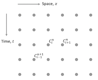
(a) Write down an expression for the central-difference approximation to the time derivative $\frac{\partial C}{\partial t}$ at the point ${C^{n+1}_i}$.
Note: The central difference approximation for the time derivative considers the time one step before, ($C^n_i$) and after, ($C^{n+2}_i$) the point of interest (${C^{n+1}_i}$), and is independent of the spacial parameter ${x}$.
(b) Explain whether the central difference approximation is more / less accurate than the forward-difference approximation.
FD: $f'(x) = (\frac{f(x + \Delta x) - f(x)}{\Delta x}) - \frac{f''(x)}{2}\Delta x - \frac{f^{(3)}(x)}{6}\Delta x^2 - ... $
BD: $f'(x) = (\frac{f(x - \Delta x) - f(x)}{\Delta x}) + \frac{f''(x)}{2}\Delta x - \frac{f^{(3)}(x)}{6}\Delta x^2 + ... $
Therefore, CD: $f'(x) = (\frac{f(x + \Delta x) - f(x - \Delta x)}{2\Delta x}) - O(\Delta x^2)... $
Hence, CD is more accurate as it's $O(\Delta x^2)$ instead of $O(\Delta x)$.
(c) Why does it become impractical to continually reduce the step-size ${\Delta x}$ in order to improve the accuracy of the simulation?
- Memory required to store values
- Finite precision of values may not be able to resolve small differences.
Problem 3.
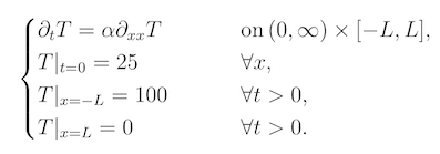
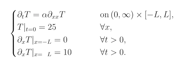
A metal bar is heated and its temperature is described by the following system of equations.
(a) Sketch the Temperature-Position graph corresponding to the bar using the following system of equations at:
(i) Initial temperature (t = 0)
(ii) At t > 0
(iii) Steady state conditions (as t tends to infinity)
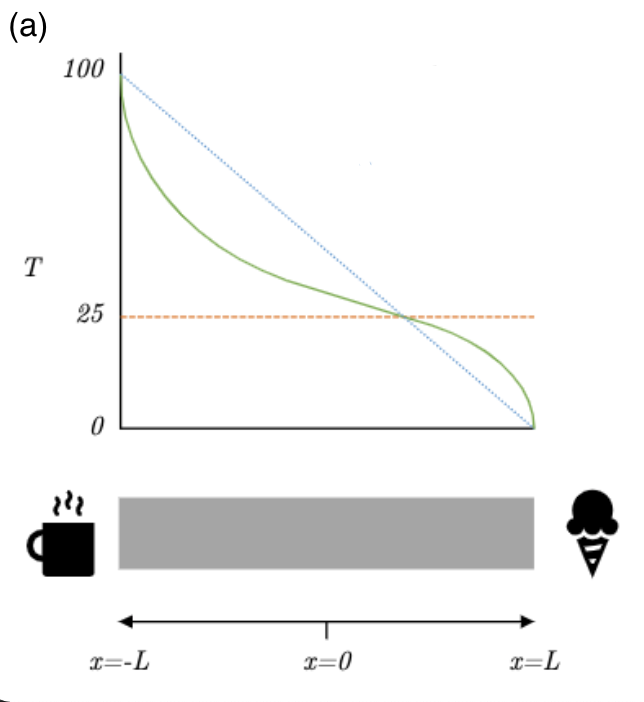
(i) Red line
(ii) Green line
(iii) Blue line
(i) At $t = 0$, the temperature is 25 degrees for all values of $x$, therefore this is displayed as a horizontal line (red).
(ii) At $t>0$ the graph will be curved (which will eventually tend towards a straight line). Ensure that the temperature is 0 and 100 at the ends of the bar (green).
(iii) The temperature will always be constant at both ends (100 degrees at one end, and 0 degrees at the other). Therefore as t tends towards infinity, this will become a diagonal line from 100 degrees to 0 degrees (blue).
Matlab Animation:
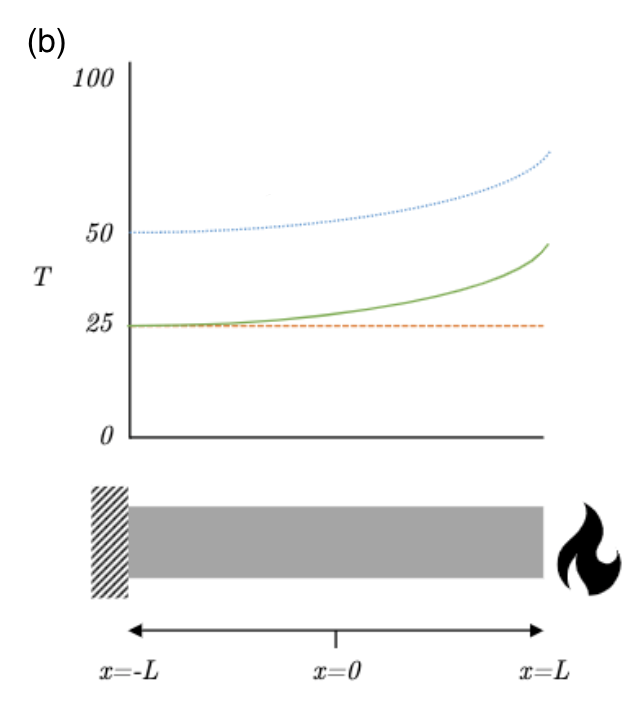
(b) Sketch the Temperature-Position graph corresponding to the bar using the following system of equations at:
(i) Initial temperature (t = 0)
(ii) At t = a (where a is some arbitrary value)
(iii) At t = b (where b is some arbitrary value and b > a)
(i) Red line
(ii) Green line
(iii) Blue line
(i) At $t = 0$, the temperature is 25 degrees for all values of $x$, therefore this is displayed as a horizontal line (red).
(ii) At $t>0$ e.g. $t=a$, the bar has a constant temperature gradient at both ends (0 at (-) end which we can think of as an insulating barrier- letting no heat in or out, and 10 at (+) end we can think of this as a controlled heat source, like a laser). Therefore the shape of the graph follows a curved shape. (green)
(iii) At $t=b$: Since this system is gaining heat at one end and not losing any heat at the other, it will keep getting hotter and hotter (shifted higher up graph), although the shape of the temperature profile will stay the same for $t≥a$. (blue)
Matlab Animation:
Extension Questions
Problem 4.
Suppose we want a one-sided approximation to $u’(x)$ based on $u(x)$,$u(x-h)$ and $u(x-2h)$,of the form: \(u'(x)\approx au(x)+bu(x-h)+cu(x-2h)\) Determine the coefficients $a$, $b$, and $c$ to give the best possible accuracy by expanding in taylor series and collecting terms.
Problem 5.
(a) Find the update equation, $x(t + \Delta t)$, of the following ODE, \(\frac{d^2x(t)}{dt^2} + \omega^2 x(t)=0\) (Hint: Use the central difference approximation to the second derivative).
Now given initial conditions of $x(0)=1$ and $\dot{x}(0)=0$:
(b) Approximate $\dot{x}(0)$ with a backward difference.
Write a table of values for $x(t)$ every $\Delta t$ time step up to $t = 2\Delta t$, using the dimensionless parameter, $\sigma = \omega^2 \Delta t^2 = 0.1$
\begin{align*} & t / \Delta t & & x(t) & \newline \hline & -1 & & 1 & \newline & 0 & & 1 & \newline & 1 & & 0.9 & \newline & 2 & & 0.71 & \newline \hline \end{align*}
(c) Approximate $\dot{x}(0)$ with a central difference.
Write a table of values for $x(t)$ every $\Delta t$ time step up to $t = 2\Delta t$, using the dimensionless parameter, $\sigma = \omega^2 \Delta t^2 = 0.1$
(d) Use Excel or otherwise to simulate both for $t/\Delta t$ up to 30, what do you see?
Answers
For Printing
Revision Questions
The questions included are optional, but here if you want some extra practice.
- Advanced Engineering Mathematics 5th edition, Stroud and Dexter : Pages 594-596 (598-605 if you’re really into the grids!)