Optimisation Tutorial Sheet, #15
Learning Outcomes
- Determine the direction towards a local minimum
- Read contour plots
- Understand costs functions
Additional Resources
Tutorials
- Excel Tutorial : How to use excel to create a residual plot.
- Accuracy of Residuals : Interesting article on residuals’ accuracy and how they are refined.
Software
- WolframAlpha : Use this to plot any function - you will become very familiar with this over the module.
In the answers, some WolframAlpha pages are linked in blue (like this)
Problem sheet
Skill Building Questions
Problem 1.
Find the line of best fit, using minimised sum squared residuals, of the form $y=mx+c$, through the following three points: (2,1), (3,5) and (7,9). Plot the resulting curve, points and residuals.
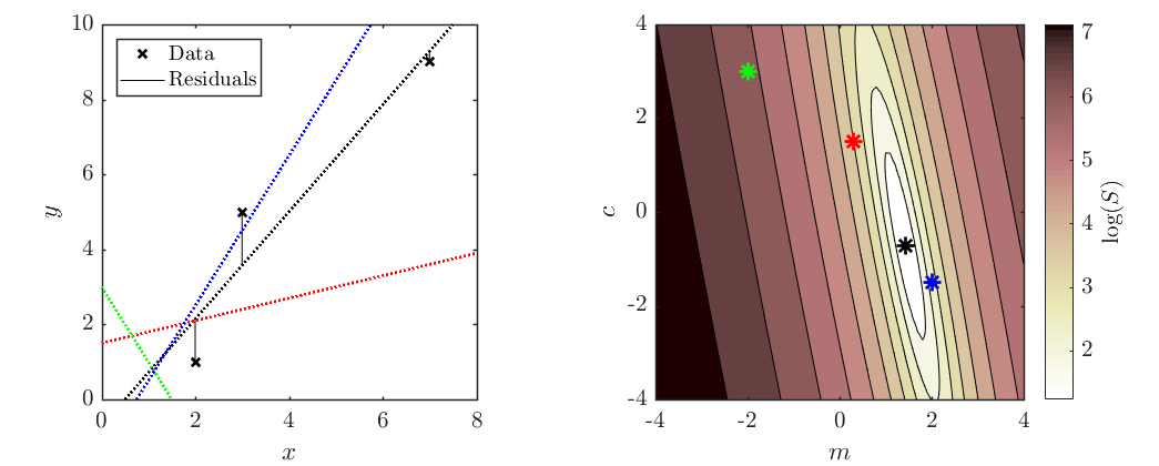 Additional lines added for the curious.
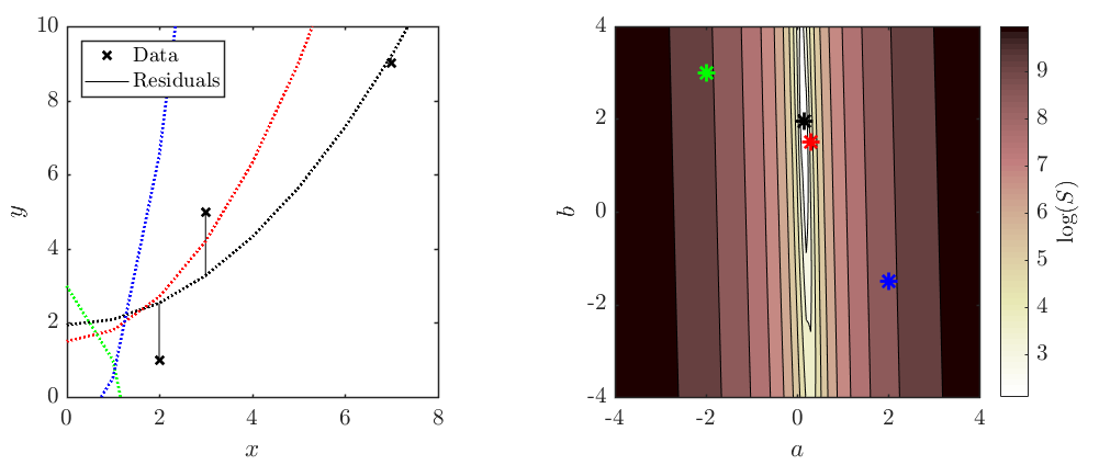
Problem 2.
Find the line of best fit, using minimised sum squared residuals, of the form $y = ax^2 + b$, through the points (2,1), (3,5), and (7,9). Plot the resulting cure, points, and residuals.
For each of the values that need to be summed or averaged from the points given in the question, we can create a table:
\begin{align*} & & &x& &y& &x_i^4& &x_i^2& x&_i^2y_i& \newline \hline \newline & & &2& &1& &16& &4& &4& \newline & & &3& &5& &81& &9& &45& \newline & & &7& &9& &2401& &49& &441& \newline & Mean& &4& &5& & & & & & & \newline & Sum& &12& &15& &2498& & 62& &490& \end{align*}
$$ a=\frac{490 - 62b}{2498} \ \ \ \therefore 2498a + 62b =490 $$ $$ b=\frac{1}{3} \times 15 - \frac{a}{3} \times 62 \ \ \ \therefore 62a + 3b = 15 $$ $$ \begin{bmatrix} 2498 & 62 \newline 62 & 3 \end{bmatrix} \begin{bmatrix} a \newline b \end{bmatrix} = \begin{bmatrix} 490 \newline 15 \end{bmatrix} $$ $$ \begin{bmatrix} a \newline b \end{bmatrix} = \begin{bmatrix} 0.1479 \newline 1.9425 \end{bmatrix} $$ $$\therefore \boxed{y=0.1479x^2+1.9425}$$
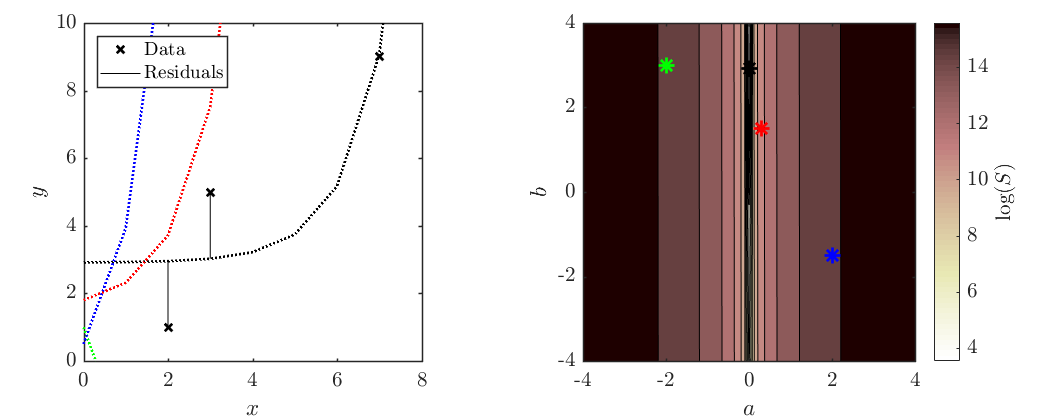
Problem 3.
Find the line of best fit, using minimised sum squared residuals, of the form $y=ae^x+b$, through the points (2,1), (3,5) and (7,9). Plot the resulting curve, points and residuals.
For each of the values that need to be summed or averaged from the points given in the question, we can create a table:
\begin{align*} & & &x& &y& &e^{x_i}& &e^{2x_i}& e&^{x_i}y_i& \newline \hline \newline & & &2& &1& &e^2& &e^4& &e^2& \newline & & &3& &5& &e^3& &e^6& &5e^3& \newline & & &7& &9& &e^7& &e^{14}& &9e^7& \newline & Mean& &4& &5& & & & & & & \newline & Sum& &12& &15& &1124& &1.2 \times 10^6& &9978& \end{align*}
$$ a = \frac{9978 - 1124b}{1.2 \times 10^6} \ \ \ \therefore 1.2 \times 10^6a + 1124b = 9978 $$ $$ b = \frac{1}{3} \times 15 - \frac{a}{3} \times 1124 \ \ \ \therefore 1124a + 3b = 1 $$ $$ \begin{bmatrix} 1.2 \times 10^6 & 1124 \newline 1124 & 3 \end{bmatrix} \begin{bmatrix} a \newline b \end{bmatrix} = \begin{bmatrix} 9978 \newline 15 \end{bmatrix} $$ $$ \begin{bmatrix} a \newline b \end{bmatrix} = \begin{bmatrix} 0.0056 \newline 2.904 \end{bmatrix} $$ $$\therefore \boxed{y=0.0056e^x+2.904}$$
 Additional lines added for the curious.
Problem 4.
The following contour plot shows the summed square error, S, for the two-parameter fit to some data for the function $f(x)=ae^{-x^2}+b$.
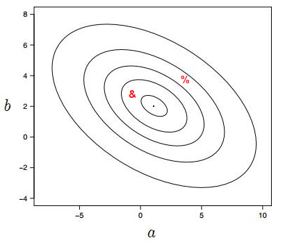
(a) Make a sketch of the curve corresponding to the best fit parameters suggested by the contour plot.
(b) On the same axis, sketch the curves corresponding to the “\&” and “\%” points from the contour plot.
(c) Add five example data points to your sketch that could reasonably have been responsible for this contour plot.
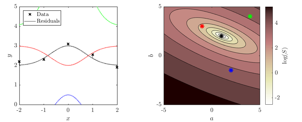
(a) Best fit parameters: $ \ \ y \approx e^{-x^2}+2 \ \ \Rightarrow \boxed{\text{Black line}}$
(b) &: $ \ \ y \approx \frac{-1}{2}e^{-x^2}+3 \ \ \Rightarrow \boxed{\text{Red line}} \quad \quad \quad $ %: $ \ \ y \approx 4e^{-x^2}+4 \ \ \Rightarrow \boxed{\text{Green line}}$
(c) $ \Rightarrow \boxed{\text{Black crosses}}$
Exam Style Questions
Problem 5.
The following sigmoid activation function, $\alpha(x)$, can be found in some artificial neural networks.
\[\alpha(x) = \frac{\omega}{\beta+e^{-x}}\]Where the “weight”, $w$, and the “bias”, $b$, are adjustable fitting parameters. To train this neuron, an engineer needs to minimise the “cost”, $C$, defined by the function
\[C(\omega,\beta) = \frac{1}{2n}\sum^n_i{(\alpha(x_i)-y(x_i))^2}\]Where $y$ is a (very small) dataset containing the three $[x, y]$ points $[0.25, -0.3]$, $[1, 0.5]$ and $[0.8, 2]$.
(a) Find expressions for the partial derivatives of $C$ with respect to each of the parameters.
(b) Calculate a Jacobian vector of the cost function, $\vec{J_C}$, at the initial point $\omega=1$ and $\beta=0$.
An easy way to calculate the Jacobian vector is using a table like the one below:
\begin{align*} & & & & &\text{wrt } \omega& &\text{wrt } \beta& \newline \hline \newline &x& &y(x)& & \frac{e^{x}(y(x)+e^{x}(-\omega + \beta y(x)}{(1+\beta e^{x})^2}& & \frac{\omega (\frac{\omega}{\beta + e^{-x}}-y(x))}{(\beta + e^{-x_i})^2} & \newline &0.25& &-0.3& & -2.03393 & &2.61162& \newline &1& &0.5& & -6.02992& &16.391& \newline &0.8& &2& &-0.501951& &1.11711& \newline & -\frac{1}{n}\sum^n_i & & \text{(mean of negatives)} & &2.855267& &-6.70658& \end{align*} -2.03393 2.61162 -6.02992 16.391 -0.501951 1.11711 Note: the blue numbers are links which will show you how the number was calculated using WolframAlpha!
$$ \therefore \boxed{\vec{J_C} = \Big[2.854, \hspace{2mm} -6.707\Big]} $$
(c) Suggest whether $\omega$ and $\beta$ should be increased or decreased to improve the fit, explaining your answer.
Problem 6.
Considering another function
\[\gamma(x) = \frac{ax}{e^x+b}\]Where $a$ and $b$ are adjustable parameters. The “cost”, $C$, defined by the function
\[C(a,b) = \frac{1}{2n}\sum^n_i(\gamma(x_i)-y(x_i))^2\]Where $y$ is a database containing the three $[x,y]$ points $[1,3.4]$, $[-2.3,0.5]$, $[2.2,-3]$, $[4.7,-6]$
(a) Find expressions for the partial derivatives of $C$ with respect to each of the parameters.
$$ \frac{\partial C}{\partial a} = \frac{\partial}{\partial a}\frac{1}{2n}\sum^n_i{\Big(\gamma(x_i)-y(x_i)\Big)^2} $$ $$ = \frac{1}{2n}\sum^n_i{\frac{\partial}{\partial a }\Big(\gamma(x_i)-y(x_i)\Big)^2} $$ Using the method that you want, determine: $$\frac{\partial}{\partial a }\Big(\frac{ax_i }{e^{x_i}+b}-y(x_i)\Big)^2 = -\frac{2x_i(y(x_i)(b+e^{x_i})-ax_i)}{(b+e^{x_i})^2}$$
Note: this can be solved easily on WolframAlpha. Link $$ \frac{\partial C}{\partial a} = \frac{1}{2n}\sum^n_i -\frac{2x_i(y(x_i)(b+e^{x_i})-ax_i)}{(b+e^{x_i})^2} $$ $$ \therefore \boxed{\frac{\partial C}{\partial a} = -\frac{1}{n}\sum^n_i \frac{x_i(y(x_i)(b+e^{x_i})-ax_i)}{(b+e^{x_i})^2}} $$
Next, solving $\frac{\partial}{\partial b }$ in a similar way:
$$\frac{\partial}{\partial b }\Big(\frac{ax_i }{e^{x_i}+b}-y(x_i)\Big)^2 =-\frac{2ax_i(ax_i-y(x_i)(b+e^{x_i}))}{(b+e^{x_i})^3}$$
Note: this can be solved easily on WolframAlpha. Link $$ \therefore \boxed{\frac{\partial C}{\partial b} = -\frac{1}{n}\sum^n_i \frac{ax_i(ax_i-y(x_i)(b+e^{x_i}))}{(b+e^{x_i})^3}} $$
(b) Calculate a Jacobian vector of the cost function, $\vec{J_C}$, at the initial point $a=0.5$ and $b=-0.5$.
An easy way to calculate the Jacobian vector is using a table like the one below:
\begin{align*} & & & & &\text{wrt } a& &\text{wrt } b& \newline \hline \newline &x& &y(x)& & \frac{x_i(y(x_i)(b+e^{x_i})-ax_i)}{(b+e^{x_i})^2} & & \frac{ax_i(ax_i-y(x_i)(b+e^{x_i}))}{(b+e^{x_i})^3} & \newline &1& &3.4& & -2.862 & &0.645& \newline &-2.3& &0.5& &27.35& &34.21& \newline &3.3& &-3& &1.615& &-0.095& \newline &4.7& &-6& &0.5172& &-0.002& \newline & -\frac{1}{n}\sum^n_i & & \text{(mean of negatives)} & &-6.655& &-8.690& \end{align*} -2.862 0.645 27.35 34.21 1.615 -0.095 0.5172 -0.002 Note: the blue numbers are links which will show you how the number was calculated using WolframAlpha!
$$ \therefore \boxed{\vec{J_C} = \Big[-6.655, \hspace{2mm} -8.690\Big]} $$
(c) Suggest whether $\omega$ and $\beta$ should be increased or decreased to improve the fit, explaining your answer.
Extension Questions
Problem 7.
Machine Learning!
When data sets are huge, Stochastic Gradient Descent can be used to find a local minimum faster. Instead of taking the sum of all data points to calculate a Jacobian (-gradient):
- Take a (random) data point
- Calculate the gradient
- Update the weights using the gradient * learning rate
- Repeat 1-3 with all data points
The method is advantageous as it makes the cost function converge faster when the dataset is large as it causes updates to the parameters more frequently.
Note: The learning rate is multiplied by the gradient to “advance” a certain distance towards the minimum. Usually, the learning rate varies because as the gradient is applied to the weights, the closer you get to the minimum and you don’t want to “overshoot” the minimum. Check out the Stochastic Gradient Descent (link in blue above) for more insight!
Considering the following function:
\[\sigma(x) = \tan^2(ax+b)\]Where $a$ and $b$ are variable ‘weights’. To determine the optimized values for these weights, the cost function $C$ needs to be minimized. $C$ is defined by
\[C(a,b) = \frac{1}{2}\Big(\sigma(x)-y(x)\Big)^2\]Where y is a dataset containing the three $[x,y]$ points $[-3,4], [2.5,6], [0.3,4.3]$ and the learning rate is $0.25$
(a) Determine the Jacobian vector of the cost function.
Tip: for the solution using WolframAlpha click on the text highlighted in blue!
(b) With the initial guess of $a = 1$ and $b=1$, determine the new weights using the first data point $[-3,4]$
Answers
For Printing
Revision Questions
The questions included are optional, but here if you want some extra practice.
- Applied/Constrained Optimisation : Overall an extension - try applied optimisation, constrained optimisation to push even further.